
FORMULA: Standard Deviation, Gauss, Normal, Binomial, Distribution

Written by Ion Saliu on October 26, 2002; later updates.
FORMULA, version 7.0, January 2003 (3 WE) ~ 16bit software.
SuperFormula ~ version 13.1, January 2011 ~ 32-bit software, superseded FORMULA.
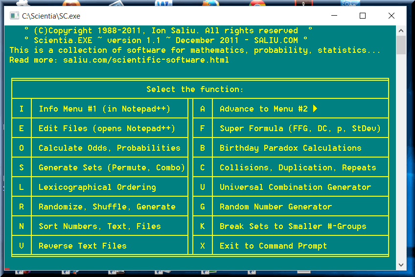
SuperFormula is now part of the most comprehensive collection of software in the fields of mathematics, probability, statistics, combinatorics: Scientia.
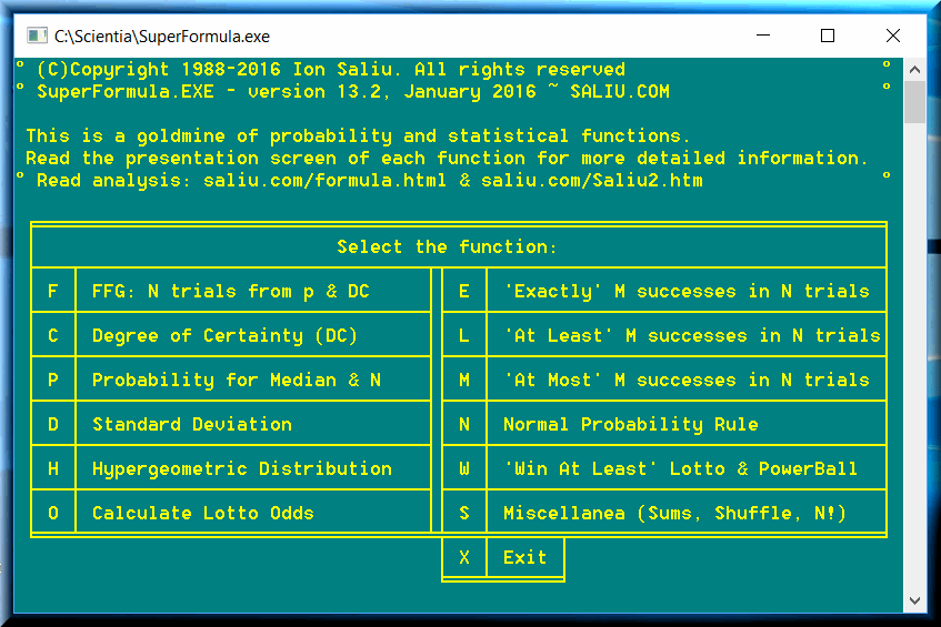
This is the definitive and the ultimate probability, gambling and statistical software.
The program boasts 12 important formulae in theory of probability and statistics:
1) The Fundamental Formula of Gambling (FFG: N from p and DC)
2) Degree of Certainty (DC from p and N)
3) Probability of FFG median (p from DC and N)
4) The Binomial Distribution Formula (BDF: EXACTLY M successes in N trials)
5) The Probability of AT LEAST M successes in N trials
6) The Probability of AT MOST M successes in N trials
7) The Probability to WIN AT LEAST 'K of M in P from N' at Lotto & Powerball
8) The Binomial Standard Deviation (BSD)
9) Normal Probability Rule (more precise than Gauss curve)
10) Calculate Lotto Odds, For '0 of k' to 'm of k'
11) Hypergeometric Distribution Applied to Lotto Odds
12) Shuffle Pools of Contiguous or Non-contiguous Numbers
I. The Fundamental Formula of Gambling (FFG: N from p and DC)
This function applies the Fundamental Formula of Gambling (FFG). It calculates the number of trials N necessary for an event of probability p to appear with the degree of certainty DC.
For example, how many coin tosses are necessary to get at least one 'heads' (p = 1/2) with a degree of certainty equal to 99%? Answer: 7 tosses.
II. The Degree of Certainty (DC from p and N)
This function calculates the degree of certainty DC necessary for the event of probability p to occur within N trials.
For example, what is the degree of certainty to get at least one 'heads' (p = 1/2) within 10 tosses? Answer: 99.902%.
III. The Probability of FFG Median (p from DC and N)
This function calculates the probability p when DC and N are known.
There are situations when you have the statistical median of a series N; therefore DC=50%; but you don't know the probability of the parameter p. The program calculates the probability p leading to a degree of certainty DC and a number of trials N.
For example, the winning reports created by LotWon software show a series of filters and their medians. If not calculated, you can use an editor such as QEdit and do a column blocking, then sort the column (filter) in descending order. The median represents the middle point of the sorted column. The median also represents the number of trials for a degree of certainty equal to 50%. I do not describe every filter in my software, so nobody can tell the probability of every filter. But you can determine it using this function of FORMULA. Other filters are described and thus their probabilities can be calculated in advance. They will prove the validity of the fundamental formula of gambling (FFG). For example, the probability of '3 of 6' in a 6/49 lotto is 1 in 57. FFG calculates the median for this situation (DC=50%) as 39. Take a real draw history, such as UK 6/49 lotto. Do the winning report for 500 past draws. Sort in descending order the filter "Threes" (or "3 #s") for layer 1. The median is 37 or closely around 39. Reciprocally, when you see a median equal to 37, you can determine the probability of the parameter as 1 in 54 (very close to the real case of 1 in 57).
IV. The Binomial Distribution Formula (BDF)
The function calculates the probability BDF of exactly M successes in N trials for an event of probability p.
For example, we want to determine the probability of getting exactly 5 "heads' in 10 tosses. We tossed the coin 7 times and recorded 5 "heads". We toss the coin for the 8th time and get another "heads" (the 6th). We must stop the tossing; the experiment failed. We can no longer get EXACTLY 5 "heads" in 10 tosses. It is obvious that the previous events influenced the coin toss number 9.
A sequence of events means that the events do not take place at the same time. They occur one after another.
The "Binomial Distribution Formula" shows some interesting facts. For example, the probability to toss EXACTLY 1 "heads" in 10 tosses is only 0.98%. It is quite difficult to get only 1 "heads" and 9 "tails" in 10 tosses.
The probability to toss EXACTLY 5 "heads" in 10 tosses is 24.6%. It is not that usual to get exactly 5 "heads" in 10 trials, even if the individual chance of "heads" is 50%! We might have thought that we would get quite often 5 "heads" and 5 "tails" in 10 coin tosses. NOT! The chance is even slimmer to get 500 "heads" and 500 "tails" in 1000 tosses: 2.52%.
The probability to get 5 "heads" in 5 tosses represents, actually, the probability of "5 heads in a row" (3.125%).
There is a data type limit. The number of trials N must not be larger than 1500! There will be an overflow if you use very large numbers. Blame the permutations and the limitations of the computers
V. The function calculates the probability of at least M successes in N trials for an event of probability p.
For example, we want to determine the probability of getting at least 4 heads in 10 tosses. Logically, the following situations qualify as 'success': 4 heads; 5 heads; 6 heads; 7 heads; 8 heads; 9 heads; and 10 heads. Obviously, the probability is better than the 'exactly 4 of 10' case.
There is a data type limit. The number of trials N must not be larger than 1500! There will be an overflow if you use very large numbers. Blame the permutations and the limitations of the computers
VI. The function calculates the probability of at most M successes in N trials for an event of probability p.
For example, we want to determine the probability of getting at most 4 heads in 10 tosses (no more than 4 in 10). In 'at least M in N' we look at the glass as being half full. Why not look at it from the pessimistic perspective: the glass can be empty sometimes (or present degrees of emptiness)! Logically, the following situations qualify as 'success': 4 heads; 3 heads; 2 heads; 1 heads; and 0 heads. The probability can be higher than the 'exactly 4 of 10' or 'at least 4 of 10' cases, but it won't be better from a player's perspective!
There is a data type limit. The number of trials N must not be larger than 1500! There will be an overflow if you use very large numbers. Blame the permutations and the limitations of the computers
VII) The Probability to WIN AT LEAST 'K of M in P from N' at Lotto & Powerball, Mega Millions
The official lotto odds are calculated as 'exactly K of M in P from N'. For example, in a lotto 6/49 game, the player must play exactly 6 numbers per ticket. The lottery commission draws 6 winning numbers from a field of 49. If the player plays only 6 numbers, the odds of getting exactly 3 of 6 are 1 in 56.66. The player can play combinations of 6 from a pool of 10 picks, for example. Now, the odds can be calculated as exactly '3 of 6 in 10 from 49': 1 in 12.75.
In real life the player gets a better deal, however. The commission does not oblige the players to 'exactly' situations. The real life situation is 'at least K of M from N'. The commissions don't care if you play just 6 numbers, or play a pool of picks. They don't care if you expected 3 of 6 hits, but hit 4 of 6. They'll pay you for the highest prize per ticket. It is clear that 'at least K of M from N' is better than 'exactly K of M from N' from the player's perspective. If the player plays 57 6-number random picks, the player should expect one '3 of 6' hit. If playing 100 times 57 tickets, the expectation should be 100 '3 of 6' hits. Sometimes, however, higher prizes can be hit. That's why the odds of getting 'at least 3 of 6 from 49' are ' 1 in 53.66'.
Many lotto wheel aficionados might broadcast screams of happiness. Cool down, Wheely! The previous calculations do not imply that 54 lines (combinations) will guarantee 100% in one draw a '3 of 6' 49-number lotto wheel! Calculating the minimum number of successes for a 100% guarantee is a totally different matter. It is a book in itself if one considers also the algorithm to generate the successes!
I wrote in the message
The Fundamental Formula of Wheeling:
the probability of winning [exactly] '3 of 6' is 1 in 57. FFG calculates the median for p=1/57 as 39.16, rounded up to 40 for DC=50%. How close is that figure (40) to reality in the UK 6/49 history file? The file I've been using for this analysis has 737 draws (contains a few so-called 'extra' draws). The file has 733 regular draws from the beginning of the game to the draw of January 1, 2003. The median for the '3 of 6' case is around 38.
The calculations are correct, as far as the standard deviation is concerned. The median, however is precisely in accordance with the probability of at least '3 of 6': 1 in 54. It's right on the money! Forget about one standard deviation! I had always noticed this small discrepancy in all the data files I analyzed. The filter medians are always a few points lower than the FFG medians. Now it fully makes sense. The medians are the result of at least K of M in N probability, NOT the exactly K of M in N probability!
We may consider from now on the Fundamental Formula of Gambling to be the most precise instrument in games theory. There are a few posts at this web site dealing with Markov chains: Suspicion is mother of the intellect; Markov chains.
Searching on Markov chains at Google yields close to 100,000 hits! The topic is hot! I stated, however, that FFG outruns Markov by several steps. Again, once and for all, the Fundamental Formula of Gambling is be the most precise instrument in games theory. Unlike Markov chains, FFG considers previous events to be of the essence for future events. The events repeat precisely, according to the Fundamental Formula of Gambling.
VIII. The Binomial Standard Deviation (BSD)
This function calculates the binomial standard deviation for binomial events (i.e., experiments characterized by two and only two outcomes: win or loss; success or failure). This is the theoretical or expected value of the standard deviation. The standard deviation can also be calculated post facto: after the experiment. Its name is self-explanatory. You can see in the WS-3 reports generated by LotWon a standard deviation for every filter. A filter goes up and down from an average value. The standard deviation calculates the positive average of all deviations (fluctuations) from an average norm.
The binomial standard deviation has great merit. It shows what fluctuation to expect. Before starting the coin toss, one can have an accurate idea of how many "heads" will come out in a number of trials (tosses). Or how many winning hands one can expect playing 200 blackjack rounds.
IX. Normal Probability Rule (more precise than Gauss curve)
When we calculated the binomial standard deviation the result is a report like this one (for 100 coin tosses):
The expected (theoretical) number of successes is: 50
Based on the Normal Probability Rule:
· 68.2% of the successes will fall within 1 Standard Deviation
from 50 - i.e., between 45 - 55
·· 95.4% of the successes will fall within 2 Standard Deviations
from 50 - i.e., between 40 - 60
··· 99.7% of the successes will fall within 3 Standard Deviations
from 50 - i.e., between 35 - 65.
The standard deviation for an event of probability
p = .5
in 100 binomial experiments is:
BSD = 5
I have been working thoroughly with pairing strategies, especially in the digit lotteries. I have encountered far better situations than offered by the traditional normal probability rule. That made me to take a different approach to calculating the normal probability rule. The traditional rule is based on Gauss or normal distribution curve. The keyword here is curve, implying continuous. The lottery or gambling are discrete, however. The one size fits all approach leads to discrepancies.
In the example above, the new normal probability rule I am using gives:
72.87% of the successes will fall within 1 Standard Deviation
from 0 - i.e., between 45 - 55
One caveat, as in the binomial distribution probability case, there is a data limit: 1500 trials. It covers a pretty good range of lottery and gambling cases.
X. Calculate Lotto Odds, For '0 of k' to 'm of k'
For example, the odds of a lotto-49 game drawing 6 numbers: '0 of 6'; '1 of 6'; '2 of 6'; '3 of 6'; '4 of 6'; '5 of 6'; '6 of 6'. The odds are '1 in 2.3', '1 in 2.4', '1 in 7.6', '1 in 56.7','1 in 1032.4', '1 in 54,200.8', '1 in 13,983,816', respectively.
The probability is calculated as exactly 'M of N' (not at least 'M of N'). Sometimes such probability is 0: the event is impossible; for example '0 of 6' or '1 of 6' for the 6/10 case.
This function handles any type of lotto game, including Keno and Power Ball. This function incorporates the entire program ODDSCALC. The program is still available as standalone.
XI. Hypergeometric Distribution Applied to Lotto Odds
This function calculates all the Odds of any lotto game, including Keno and Powerball, using the hypergeometric distribution probability.
For example: In a lotto-49 game drawing 6 winning numbers, what are the odds of getting exactly '1 of 6' when the player plays 6 numbers, AND the lottery draws 6 numbers from 49. In the case above: the probability of (1,6,6,49); or (4,6,6,49); or (10,10,20,80 - Keno) . . .
This calculator helps to figure out the odds when playing combinations of various lengths and for various prizes.
This function incorporates the entire program ODDS. The program is still available as standalone.
XII. Shuffle Pools of Contiguous or Non-contiguous Numbers
SHUFFLE can shuffle (randomly arrange) a group of contiguous numbers from 1 to N. If the user types 10 at the input prompt, the program will start a continuous process of randomizing 10 unique numbers, from 1 to 10. The sequences look like: 3, 7, 1, 9, 10, 4, 6, 5, 2, 8. The sequence 1, 2, 3, 4, 5, 6, 7, 8, 9, 10 is so rare that it is said only Almighty Number can generate it.
There is another situation: groups of non-contiguous numbers, such as: 1, 44, 33, 55 77 22 66 99 13 111 49 29 25 9 54. Function XII of FORMULA can handle this type of randomizing situations as well. The groups of non-contiguous numbers can be typed at screen prompts. Or, the numbers can be saved to a text file first. The text file can be used as an input device to FORMULA. The numbers must be separated by space(s), or commas, or combination of both. Also, the numbers can be placed on several lines, or in one column. The user chooses how many times to run the randomization process. The initial group of non-contiguous numbers can be arranged in any order, including sequential.
"As we walk in steps and speak in words, so the Cosmos moves in laws and thinks in formulae."
(Axiomandros of Agrimmas, "On Ionian Pillars")
"For only Almighty Number is exactly the same, and at least the same, and at most the same, and randomly the same. May Its Almighty grant us in our testy day the righteous proportion of being at most unlikely the same and at least likely different. For our strength is in our inequities."
Resources in Theory of Probability, Mathematics, Statistics, Standard Deviation, Software
See a comprehensive directory of the pages and materials on the subject of theory of probability, mathematics, statistics, standard deviation, plus software.
Comments:
Home | Search | New Writings | Software | Odds, Generator | Contents | Forums | Sitemap