

I. Introduction to Standard Deviation: Fluctuation in Random Phenomena
II. Binomial Standard Deviation
III. Statistical Standard Deviation
IV. The Best Software to Make Sense of Standard Deviation (Evaluation)
V. Meaning of Standard Deviation: Dispersion, Volatility, Control Over Data
VI. Standard Deviation and Chi-Squared Distribution
VII. Fundamental Formula of Gambling (FFG): The Most Precise Instrument in Randomness
VIII. Resources in Theory of Probability, Mathematics, Statistics, Standard Deviation, Software
Furthermore, the results of a random (or probability, or stochastic) event can be defined as a data series (or a statistical series). All data series show variation, or variability, or fluctuation. Although some elements may be equal to one another, many elements differ in value.
Fluctuation or variation can be measured by several methods. The most common method measures fluctuation in rapport to:
~ the expected value of the event
~ the mean average of a data series.
The elements of a data series vary from the expected value or the average by positive or negative quantities. The two methods lead to the well-known parameter named standard deviation.
The standard deviation is viewed as:
~ a probability parameter of binomial events (compared to the expected value)
~ a statistical parameter of a numerical series (compared to the mean).
Standard deviation = SQR{(N * p * (1 - p)}
where p is the probability of appearance and N represents the number of trials,; SQR, a programming term in Basic, means square root or radical √.
Suppose we toss a coin 100 times (N=100). The probability of heads is p = 1/2 = .5. The standard deviation is SQR{100 * 0.5 * 0.5} = square root of (100 * .25) = √25 = 5. The expected number of heads in 100 tosses is 0.5 * 100 = 50. The rule of normal probability proves that in 68.2% of the cases, the number of heads will fall within one standard deviation from the number of expected successes (50). That is, if we repeat 1000 times the event of tossing a coin 100 times, in 682 cases we'll encounter a number of heads between 45 and 55.
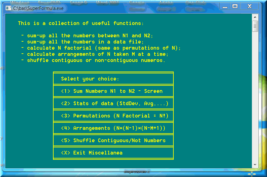
Super Formula calculates the binomial standard deviation AND the statistical standard deviation of any numeric data series.
~ the binomial standard deviation: Option D;
~ the statistical standard deviation: Option S = Miscellanea (Sums, Shuffle, N!, Standard deviation), then 2 (Stats of data: Standard deviation, mean average, median, sums).

The numbers (small or huge, integer or floating point) are first collected in a file (ASCII or text format). The program also calculates the sum; mean average; minimum and maximum values. The statistical standard deviation validates the binomial (probability) standard deviation. Moreover, the FFG (non-standard) deviation more closely fits real data. The reality follows closely the theoretical laws.
One serious problem with the standard deviation as an analytical tool: It is distorted by extreme values (extremely high, or extremely low) in the data series.
Here is an example of a data series saved in a lotto 5/39 game file (Pennsylvania lottery Cash 5):
The Sum of 13,825 numbers in \LOTTERY\LOTTO-5 is: 276,423
Mean Average: 19.99
Standard Deviation: 11.29
Median: 20
Minimum: 1
Maximum: 39
The data file can be created easily in any text editor, including MDIEditor Lotto WE. The file can have uneven lines; i.e. variable numbers of items per line. Or, the data file can consist of one huge column; i.e. one number per line. The numbers can be separated by spaces, commas, tabs, or [Enter]. You can also export data from spreadsheets or databases to text files.
But how do we define the standard deviation as being good, or acceptable, or normal? By many standards, a large standard deviation indicates a non-desirable dispersion of the data, or a wide (wild) spread. It is said that such a phenomenon is very volatile. Volatile phenomena are much harder to analyze, or define, or control.
I haven't found in the literature numerical or statistical parameters to define a good standard deviation. I have come up with my own standards. A phenomenon is not negatively volatile (or a phenomenon has a good dispersion) if the standard deviation measures closely to the mean average or the median of the data series.
Believe it or not, the lottery, the roulette, the blackjack are not very volatile. Here is an exemplification for the double-zero roulette:
Sum of 1000 numbers in SPINS00.DAT is: 19406
Average: 19.41
Standard deviation: 10.77
Median: 19
Minimum: 0
Maximum: 37 (00)
On the other hand, horse racing is very volatile. Take as good example the trifecta payouts.
Total trifectas (triactors): 236
Total amount paid for trifectas (triactors): $170,396.35
AVERAGE trifecta (triactor) payout: $722
Standard deviation: 2349.25
Minimum trifecta (triactor) payoff: $17.80
Median trifecta (triactor) payoff: $221
Maximum trifecta (triactor) payoff: $26,914 (Belmont Park).
The standard deviation is more than three times greater than the average and more than 10 times larger than the median. The payouts are strongly influenced by the number of horses in the race (from four, even fewer, to 14 horses or more). Also importantly, if the betting favorites are in top three finishers, the trifecta payouts are disappointing; if long shots win, the trifecta payouts skyrocket!
The stock market is also a painfully volatile phenomenon. The high tech bubble burst of the year 2000 is still a painful memory in the United States. The standard deviation in the stock market can be sky high sometimes, compared to the mean average or the median. Unfortunately, extreme volatility does kill hope, to say the least.
I prefer the normal probability rule to determine the independence of a data series. Let's use the same example of 6/49 lotto game. The degree of certainty is equal to 99.8% that every lotto number will have a frequency between 2 and 22 in any 100 draws. That is, 3 standard deviations from the expected frequency of 12.
Roulette is a totally different game.
In the case of an event of probability p = .02631579 (1/38) in 100 trials:
The expected (theoretical) number of successes is: 3
Based on the Normal Probability Rule:
· 68.2% of the successes will fall within 1 Standard Deviation from 3 - i.e., between 1 - 5
·· 95.4% of the successes will fall within 2 Standard Deviations from 3 - i.e., between -1 - 7
··· 99.7% of the successes will fall within 3 Standard Deviations from 3 - i.e., between -3 - 9
Real life roulette spins will show that some numbers do not come out in 100 spins, or more. There are situations when a roulette number is not drawn in over 200 spins!
The normal probability rule indicates a very important factor: What is the minimal number of trials to meet a degree of certainty (or a level of confidence)? In the roulette case, 100 spins are not sufficient to meet a 95% degree of certainty. Negative values for the lower bound mean that the level of confidence cannot be satisfied. The maximum satisfied is 88.15%.
In the case of an event of probability p = .02631579 (1/38) in 100 trials, 88.15% of successes will fall within 3 standard deviation(s) from 3; i.e. between 1 and 5; the standard deviation is: 1.60073.
Many use the standard deviation or chi-square to describe the fairness of a phenomenon, especially in the gambling field. Analysts use the standard deviation or chi-squared to make sure that roulette, for example, or the lottery is not rigged (fixed). The standards themselves, however, are wildly dispersed and volatile
The FFG median represents the number of trials N for a degree of certainty DC equal to 50%.
Each and every random event repeats, in at least 50% of the cases, after a number of trials less than or equal to the FFG median.
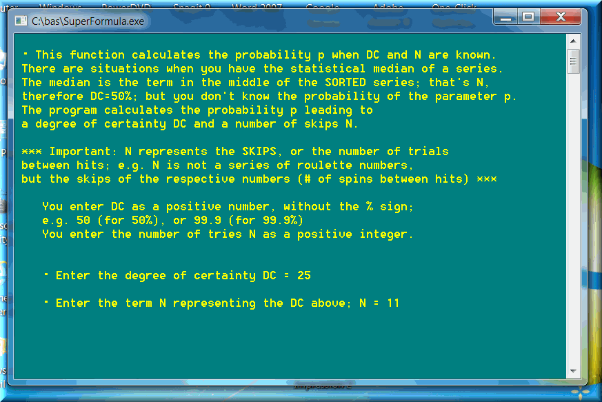
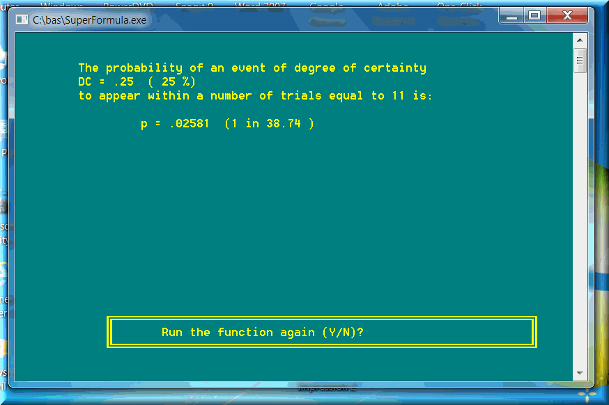
We can go one step further and apply the Fundamental Formula of Gambling to calculate another valuable probability and statistical parameter: the FFG deviation. The FFG deviation represents the number of trials N for a degree of certainty DC equal to 25%. If we know the probability p of an event, we can easily determine the deviation by simply applying FFG for a DC = 25%. Take the American roulette (double-zero) as an example. The probability p = 1/38. The FFG deviation is equal to 11. I checked real roulette spins or thousands of random spins. The statistical standard deviation of data is always mathematically equal to FFG deviation: 11. You can take it to the bank
It is for the first time in mathematics that we can determine the standard deviation of a phenomenon IF we know its probability p. I have checked a statistically-valid large number of cases: FFG deviation is always mathematically close in value to the statistical deviation.
The reverse is also valuable. If we have a large data series, we can determine the standard deviation. From there, we can determine, with very good approximation, the probability of the event. We simply apply Super Formula, function P = Probability for Median and N. In this case, median simply refers to the degree of certainty DC equal to 50%. In fact, you can enter ANY DC you want. In our case here, DC = 25%. The result will be a probability value p very close to mathematical reality.

Again, we need a large data series, as large as to satisfy Ion Saliu's Paradox of N Trials. Say, probability p = 1/N. If we have a data series with a number of elements (N * 20), we are extremely close to certainty. Take the American roulette, where p = 1/38. Just 38 * 20 = 760 roulette spins will definitely satisfy the requirements of precision in calculations.
If you have 760 American roulette spins, you can bet baby milk money that the statistical standard deviation is 11. Or, after you determine that standard deviation is really 11, the probability p will be really close to 1/38. Take any numbers you get real casino spins or randomly generated numbers. Write roulette numbers as they are: 17, 8, 29, 36, 0 The double-zero will be written as 37.
Thus, if we have a significantly large number of sales figures on a daily basis, we can determine a quite accurate probability of daily sales.
You'll read next a reference to Chebychev's Theorem or Inequality. That theorem must definitely be surrounded by sarcastic quotation marks: It is extremely lax! The normal probability rule was derived from that theorem and it attempted to be more precise. The normal probability rule is still lax too generous or too cautious, that is. After N * 20 cases, the degree of certainty is as close to the mathematical probability as a tiny fraction of just one standard deviation! Forget all together about three standard deviations that's too huge of a margin of error!
Disregard the screen text: The calculations do apply to real roulette numbers as well (not only the skips)! As you can see on the next screenshot, the probability p is a little lower mainly because FFG mixes integers with floating-point numbers. In this case, a standard deviation equal to 11 was a rounded integer from a floating-point number.
It doesn't depend on size, or a cow would catch a rabbit.
(Pennsylvania German Proverb, from Warren Weaver's excellent book "Lady Luck", chapter IX, "Variability and Chebychev's Theorem")

 Read Ion Saliu's first book in print: Probability Theory, Live!
~ Discover profound scientific implications of the Fundamental Formula of Gambling (FFG), including mathematics, Statistics, standard deviation and FFG deviation.

Of major interest:

Home | Search | New Writings | Fundamental Formula | Odds, Generator | Contents | Forums | Sitemap
